George Broyles, Forestry Technician

Abstract

This web-based version of TabGen was written to produce tables of results using Forest Inventory and Analysis (FIA) data. In addition, TabGen computes sampling errors for each cell in each table (MapMaker approximates these variances rather than computing them directly). The approach to estimation is described along with some common misunderstandings of how to use FIA data. The development of the correct estimates of forest area, attribute totals, and their means over the area of interest is described. Program TabGen was written to perform these calculations assuming simple random sampling, stratified random sampling, or double sampling for stratification.

Introduction

The results of forest surveys generally are produced in the form of one- and two-way tables. For example, forest managers and planners may make decisions based on tables of the area by forest type and stand size or volumes by species and diameter class. The statistical reports of the Forest Inventory and Analysis (FIA) units of the USDA Forest Service are compilations of such tables. Although we regularly use such tables, the forest survey and sampling literature describes sampling designs and alternative estimators for a single attribute of interest rather than for tables of them.

There is confusion over how to construct tables involving a measured variable, e.g., volume, which is then divided into rows and columns by categorical variables, such as stage of development and site class. Typically, the table total is divided into rows that are further broken down into columns. These values are not unrelated estimates because they must add across and down. The literature does not address this issue directly. Sometimes additivity constraints are imposed after estimating each cell independently (Li and Schreuder 1985). For the sampling designs and estimators described here, the tables are constructed to be additive (except for ratio estimators). Because cells are estimated independently, there often is confusion over the sample size of each table cell, which then affects the estimate of precision for that cell.

In many forest surveys, especially in the United States, there is interest in estimating not only various forest characteristics but also forest-land area. This requires sampling the entire land area and then estimating the portion that is forested. This creates confusion in sample sizes and in how to express the values as totals and on a per-unit-area basis.

This paper presents estimators for construction tables of values and their variances. The estimation steps presented are designed to avoid some of the confusion and mistakes described previously. These procedures have been incorporated into this web-based version TabGen.

Methods

The first step in clarifying the estimation of tables is to present the estimators in the context of estimating tables. This is done at some length in this section to set the stage for addressing sources of confusion such as sample size, estimation of forest area, and expressing values on a per-unit-area basis.

Estimation

Typically, estimators are derived for a single attribute of interest, for example, total biomass of a forest. When estimating tables, one may be interested in estimating biomass by species group and diameter class. The estimation process is the same for each cell--only the attribute of interest changes. Alternatively, the estimation process and the attribute of interest are the same in each cell but different conditions are placed on the attribute of interest in each table cell. The latter approach is taken here.

Each row and column category can be thought of as a condition to be placed on the attribute of interest. Row and column variables must be categorical or must be continuous variables that have been divided into classes, e.g., diameter classes. The attribute of interest is "summed" into a cell only when it meets the row and column conditions. Each categorical variable has an associated indicator variable-- either the attribute is in the category of interest (1) or it is not (0). For example, when estimating the volume in Site Class 3, if the Site Class for the sampling unit (plot or cluster of plots) is 3, the indicator variable for the sampling unit is assigned as 1, otherwise it is 0. So for each cell, indicator variables can be assigned to an observation for each categorical variable (row and column variables)--either the observation belongs in that cell or it does not. This method is described in Cochran (1977, p. 142- 144) for estimating domain (cell) means.

These indicator variables can then be used in the estimation process. Because values of 0 and 1 were chosen, the indicator variables can be multiplied times the attribute of interest for each observation. If either the row or column indicator is 0, the product of the two indicator variables and the attribute of interest is zero. This product is then averaged across all sampling units within each stratum. In the simple random sampling case, this is the final estimate because simple random sampling can be thought of as stratified random sampling with a single stratum. However, stratification often is used to reduce the variance of the estimates by subdividing the population into relatively homogenous strata. In this case, the strata means are averaged using the stratum areas as weights (stratified random sampling estimator) or using estimated stratum weights (double sampling for stratification). The variances also are computed using the product of the attribute of interest and the indicator variables.

The formulas that follow assume stratified random sampling where strata are defined on maps or satellite imagery. Examples include map-based forest type, stand-density classes, and land-use classes. The simple random sampling formulas are the same except that there is only one stratum. Double sampling for stratification (Cochran 1977) estimators are the same except that an additional terms are added to the variance because stratum areas also must be estimated (see also Chojnacky 1998).

Examples include photointerpreted land-cover classes, or volume classes.

The population mean (per unit area) for the attribute of interest in row, r, and column, c, is estimated as:

where:

• Nh = area (or count) in stratum h, where h=1, 2, ..., H
• N = total area (or count) in population (across all H strata)
• nh = number of sampling units observed in stratum h
• Yhi = attribute of interest (expressed on a per-unit-area basis) on sampling unit i in stratum h. For example, the sum of tree observations divided by their plot area.
• Ihir = indicator variable for row r of the first categorical attribute of interest for sampling unit i in stratum h. Equals 1 if the value of the attribute matches row r, and is 0 otherwise.
• Ihic = indicator variable for column c of the second categorical attribute of interest for sampling unit i in stratum h. Equals 1 if the value of the attribute matches column c, and is 0 otherwise.

In other words, the products of the attribute of interest, Yhi, and the two indicator variables are summed over all sampling units in a stratum and divided by nh to form the strata means. These means are combined using the stratum weights to form an estimate of the population mean for each cell (r, c) in turn. No matter the value of Yhi, the contribution of a sampling unit is 0 if either of the indicator variables, Ihir or Ihic, is zero.

To estimate the proportion of the area in each table cell (combination of r and c), the attribute of interest in equation (1) becomes the proportion of plot i in the condition of interest, Ahi:

The estimated variances are computed from Cochran (1977, eq. 5.12) as:

and,

where:

• Yhirc = product of attribute of interest and the indicator variables = Yhi Ihir Ihic
• Ahirc = product of the area attribute of interest and the indicator variables = Ahi Ihir Ihic

To estimate population totals such as total volume or area of Site Class 3, multiply equations (1) and (2) by the known total area in the population, AT. Their estimated variances are then equations (3) and (4) multiplied by AT 2.

If simple random sampling is used, then H = 1 and Nh = N. If double sampling for stratification is used, Cochran (1977, eq. 12.32) replaces equations (3) and (4). Note that equations (5) and (6) simplify to (3) and (4) if the total number of first-phase samples (usually interpreted on aerial photographs), N, equals the total area, AT.

and,

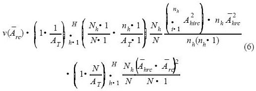
where:

• Nh = number of first-phase samples that fell in stratum h
• N = total number of first-phase samples taken to determine strata areas

These equations are all that is needed to construct tables of means for an attribute of interest and for area proportions, and to create tables of their variances under simple random sampling, stratified random sampling, or double sampling for stratification designs.

Sample Size

Note that for estimates of all cells, the sample sizes, nh, have remained the same. Often, survey analysts assume that the sample size is the number of sampling units that "fell" into a cell, that is, the number of sampling units for which both indicators were 1. Mathematically, this is the sum of the products Ihir Ihic. This sum is a random variable--it was not known (fixed) in advance of sampling (as was the sample size, nh). In fact, when the sum is divided by the sample size, it forms an estimate of the proportion of sampling units falling in the cell of interest, which is a random variate (we can estimate its variance in (4)). Another way to understand this is that all attributes of interest are observed on all sampling units but that often the observation is zero.

Often, interest is in the mean of an attribute of sampling units falling in a cell. Unfortunately, the mean estimated in equation (1) is the mean based on all sampling units. Often, these means are difficult to interpret, such as the average volume per acre that includes both forest and nonforest acres. Thus, estimates using equation (1) generally are transformed by multiplying by the total area, AT, to yield totals across the population. Further, these totals can be divided by the estimated area in each cell resulting in an estimate of the mean of an attribute for sampling units falling in a cell, as shown in the following section.

Expressing Values on a Per-Unit-Area Basis

Often, interest is in the mean of observations falling within a particular cell, expressed on a per-unit-area basis, such as the volume per hectare of pine in pine plantations versus the volume of pine on an "average" hectare across the whole forest, as is given by equation (1). Rather than using only sampling units that fall in the cell of interest, all sampling units are used--first to estimate the total volume of pine in pine plantations and then to estimate the total area of pine plantations. Dividing the total by the area then gives a slightly biased (of order 1/n) estimate of the attribute of interest on a per-unit-basis for the area of interest. This is equivalent to dividing the mean across the whole forest (1) by the proportion of the area in the class of interest (2):

The approximate variance of this combined ratio-of-means estimator (Cochran 1977, eq. 6.51) is:

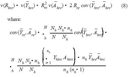
Note that a single estimate of the ratio is used rather than one for each stratum. Analogously, an approximation to the estimated variance in the double sampling for stratification case is:

This process is repeated for each combination of the categorical variables, plus the total across all classes (row and column margins). This provides all of the formulas needed to construct a variety of tables for attributes of interest, area, and the ratios between the two. Note that if estimates are to be placed on a per-observation basis, e.g., per-tree, Ahi values should be replaced with the number of observations per acre.

Estimation of Forest Area

Forest inventories for an ownership typically are map based and only forest areas are sampled. In regional forest inventories such as FIA, no maps of all forested areas are available, so forest area must be estimated from the sample. The forest area is estimated easily using equation (2). The categories of interest are forest and nonforest. The proportion of sampling units falling in forested conditions times the total land area sampled, AT, yields an estimate of the total forest area. Since remaining tables would focus only on the forested sampling units, it is tempting for the analyst to only use the forested sampling units in further analyses. However, the number of forested sampling units is a random variable, so all sampling units must be included in all analyses. This is done using the methods described earlier. FIA often presents the results as totals, AT times equation (1) to simplify the estimation. Means across forest and nonforest areas, as given in equation (1), are rarely useful; means generally would have to be estimated using equation (7) with total forest area or some subset of it as the denominator. This is more complicated because it uses equations (1)-(4) and (7)-(9), rather than only (1)-(2).

Program TabGen

To avoid these complexities and confusion, program TabGen (Table Generator) was developed. TabGen allows the user to create tables in a web environment. It uses all the formulas presented here and avoids the pitfalls mentioned.

Currently, the program reads a modified version of the FIADB (Miles et al 2000). The modifications included the addition of a field to identify each plot's stratum, plus a table of stratum weights, and another of the total area in each population (county). The FIADB includes data on the following: plot (sampling unit) data, area condition, regeneration, and overstory trees. TabGen also reads a control file that contains a list of plots to be included in the analysis. This list potentially allows the analyst to include only the subset of plots of interest, such as for a user-defined polygon.

TabGen reads a variable library (dictionary) that describes the variables that are read from each file, whether they are continuous or categorical, and, if categorical, the labels for each category. The user then selects the row, column and page categorical variables and the attribute of interest (continuous variable). The results can be viewed as:

1. The percent of the area or total area in each cell--equation (2)
2. The mean or total of the attribute of interest in each cell--equation (1)
3. The ratio of the mean to the area estimate for each cell--equation (7)
4. The mean of individual observations (generally on a per-tree basis)
5. The number of plots "falling" in each cell

The 95% sampling errors (confidence limits) are given for each cell:

where:

• t = Student's t-value with á = .05 and nh degrees of freedom. As nh goes to infinity, t goes to 1.96; thus, 2 is substituted.
• V = variance estimate of the mean

The estimates and their variances are computed using simple random sampling, stratified random sampling, or double sampling for stratification estimators.

TabGen generates two- or three-way tables. Filters can be used to create rules for a variable that determines which plots or observations will be included/excluded from the analysis. Multiple filters can be created for each variable. For example, a tree-size filter can be created from DBH. A table of volume by species and site class can be created first for poletimber trees and then for sawtimber trees. Filters also can be used in combination, for example, adding a filter only for pine plantations.

Acknowledgements

Mead Paper Corp. and the USDA Forest Service, San Dimas Equipment Development Center provided financial support. Chip Scott, Scott Klopfer and Pat Miles did the programming for TabGen.

Literature Cited

Chojnacky, D.C. 1998. Double sampling for stratification: a forest inventory application in the Interior West. Res. Pap. RMRS-RP-7. Ogden, UT: U.S. Department of Agriculture, Forest Service, Rocky Mountain Research Station. 15 p.

Cochran, W.G. 1977. Sampling Techniques. New York: John Wiley & Sons. 428 p.

Li, H.G.; Schreuder, H.T. 1985. Adjusting estimates in large two-way tables in surveys. Forest Science 31: 366-372.

Miles, P.D.; Brand, G.J.; Alerich, C.L.; Bednar, L.F.; Woudenberg, S.W.; Glover, J.F.; Ezzell, E.N. 2001. The Forest Inventory and Analysis Database: Database Description and Users Manual Version 1.0. Gen. Tech. Rep. GTR-NC-218. St. Paul, MN: U.S. Department of Agriculture, Forest Service, North Central Research Station.

Note: this documentation was based on:

Scott, C.T. 2000. Estimating two-way tables based on forest surveys. Proc. Integrated Tools for Natural Resources Inventories in the 21st Century. Burk, T.E. and M.H. Hansen, ed., Boise, ID. USDA Forest Service, North Central Research Station, St. Paul, MN. GTR-NC-212. p. 234-238.