

National Agricultural Imagery Program Prep Imagery Help
NAIP Prep Imagery User Guide (PDF, 1 MB)
Overview
The NAIP Prep Imagery (NPI) application is a National Agricultural Imagery Program (NAIP) image preparation tool to run Google Earth Engine (GEE) bioclimatic (BIOCLIM) models. It uses the collected training points captured in the NAIP Digitizing Tool (NPD) sister application.
National Agricultural Imagery Program (NAIP) is high resolution ‘leaf-on’ imagery flown for the United States Department of Agriculture (USDA).
The user interface is a series of steps that are used to help setup an area for modeling. Additionally, the Graphical User Interface (GUI) is used to streamline running the model during each session. The GUI serves the purpose of gathering parameters to send to the processing software.
The application is a Single Page Application (SPA) reactive GUI that allows for a better User eXperience (UX) where parts of the interface are updated without a sequence of screens.
This application is run in the Google Earth Engine (GEE) site at code.earthengine.google.com. GEE is a web-based Interactive Development Environment (IDE) for the Earth Engine JavaScript API. GEE code editor features are designed to make developing complex geospatial workflows fast and easy.
The GEE site also features a large set of geospatial data and a repository for user created data. The site automatically brings more servers into service as needed without any coding.
The objective of this document is to introduce and describe the use of the Forest Health NPI application in GEE. The application’s purpose will help to minimize any ‘behind the scenes work’ in the GEE script window and to allow for more defined adjustments and protocols for obtaining model results.
Acronyms and Abbreviations
| ABBREVIATION | ACRONYM |
|---|---|
| BIOCLIM | Bioclimatic Prediction and Modeling System |
| CSV | Comma Separated Value |
| FAQ | Frequently asked questions |
| GEE | Google Earth Engine |
| GUI | Graphical User Interface |
| IDE | Interactive Development Environment |
| NAIP | National Agricultural Imagery Program |
| NNS | NAIP Native Scale |
| NPD | NAIP Point Digitizing |
| NPI | NAIP Prep Imagery |
| SPA | Single Page Application |
| TCH | Tree Crown Health |
| USDA | United States Department of Agriculture |
| UX | User eXperience |
Background
The Forest Service has been using GEE for remote sensing and risk mapping processes. The scripts written for GEE were developed in the JavaScript programming language. The scripts were developed for viewing aerial imagery and extracting data (point digitizing) from that imagery. The points and data obtained via the digitizing process are later input into a model that gives predictions for tree crowns or canopies that are either healthy (live) or unhealthy (dead or dying).
The resulting maps provide nation-wide assessments of forest health. The maps highlight areas affected by insects and disease. The accuracy of these models and maps are influenced by the quality and quantity of training points, and the quality of the NAIP imagery.
Many variables can sway the model into picking up non-treed areas. The soil/understory can be similar to red tree crowns (early stages of mortality). Gray canopies (later stages of mortality) can also share similar spectral characteristics to rocky outcrops and bare soil. Post processing methods, involving masking layers, are used to minimize confusion between trees and other features such as the forest understory.
Contents
The purpose of this code is to gather parameters and select training points for input into the model and output resulting model imagery and points as layers and optionally as an asset on permanent storage.
1-Select a State and Year
The state and year of the desired points are captured in this section.

NAIP imagery is collected approximately every other year for each state. However, Alaska, District of Columbia, Hawaii and the territories are not included. The NPI application models points on the NAIP imagery for a state and year (and incidentally an ecoregion) acquired from the NPD application.
Click the ‘Select a value’ box to choose a state where digitized points exist.

Selecting a state will zoom to the state, center the map in the map window, populate the ‘Select a NAIP Year’ and list the year(s) available for the selected state while automatically selecting the most recent year. Be patient while the display is updated.

After selecting a state, click ‘Select a NAIP Year’ to select one of the available years for the state and display the points. The most recent year is the first choice in the descending ordered list. The year may show as a negative value when another state is selected with the same most recent year. The negative sign is only to trigger an on-change event to gather new points. This will occur if you switch between states in the same browser session of the application. Rerunning the application will ‘fix’ it.

2-Prep Imagery Info
Additional information about parameters for the model are captured in this section.

ECOREGION
Some states such as California are very diverse ecologically. This means there’s many different soil types, vegetation, and topography across the entire state. Filtering training points by an ecoregion can help to minimize commission and omission errors that may occur from state wide model results. The model output will only overlay in the selected ecoregion and derive the training points within its boundary.
Checking the box causes an ecoregion layer to display.
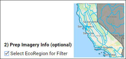
An ecoregion can then be selected with the cursor. Once selected, the ecoregion polygon will highlight orange and the ecoregion ID is added to the display and map layers. This ecoregion ID will also be indicated in the saved output file name.

SCALE
The scale for the output BIOCLIM map can be adjusted on the slider. This will establish the cell size for the reduced resolution output BIOCLIM map. Running the model will always include Naip Native Scale (NNS), and the chosen selected cell size value. The value selected on the slider is shown in the map layers.
FHAAST uses standard snap grids at 30, 240, 480, 960, and 1920 m. In NPI, when a scale that is coarser than NNS is used, it will typically be 30 meters.
Click and drag the square box along the slider to change the output cell size in meters. By default, it’s always set to 30 meters.

The scale slider can select values between 3-30 meters in increments of 3.

THRESHOLD
The threshold tolerance establishes the minimum number of points required for each color class to participate in the model. If the number of points does not meet the threshold a constant band of zeros are output for the band. Note that each color does not operate in isolation and additional colors contribute to the minimum tolerance for including the color. An example would be: In order to generate a Gray model output, it must have either Red or Absence training data. If Red or Absence points don’t exist, then a gray model can’t be computed or viewed on the map.
| COLOR | ADDITIONAL COLORS CONSTRAINT |
|---|---|
| Red | Gray Absence |
| Green | Absence Shadow |
| Gray | Red Absence |
| Absence | Red Gray |
| Shadow | Green Absence |
The value selected on the slider is used in the model and the tolerance value is included in the layer name and the saved output file.
ENVELOPE
The nine envelopes (60, 70, 80, 90, 96, 100, 104, 110%, and Optimal) are used to both visually and statistically “tune” the model outputs against the NAIP imagery. As a default, Optimal is used to let the model compute an envelope. It chooses based on accuracy and kappa statistics. Simply put, it’s selecting the ideal envelope that has the least overlap between two or more model output colors.

Selecting each color ‘Env’ button will display its own dropdown list. Note: during the model evaluation process, it’s best to leave the ‘ENV’ dropdowns untouched. By default, the envelope will be set to ‘Optimal’. This is crucial in seeing how the model results look firsthand and will allow for a good baseline to see if a lower or higher envelope may be better desired.

After choosing a desired envelope, the dropdown list will close, and the selected value will display in the box.
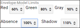
In order to understand how to adjust the model envelope, it’s important to assess the outputs on the map first. The Envelope-Model Limits can help to limit model outputs from over or under prediction i.e. (commission and omission errors).
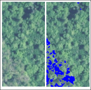
This scenario is an example of fine-tuning Gray commission errors and the same method can be applied for the each of the five color classes. The optimal envelope here was set to the maximum threshold at 110%. Begin by seeing how it outputs on the map.
The 110% envelope is too inclusive for a reliable and accurate model. In this case optimal isn’t mapped well here. It’s predicting within all the surrounding green tree canopies as well as the mortality in the bottom left. Be sure to look at the 2m view scale to see how it’s outputting against individual Naip native scale pixels.

Start by lowering the model envelope threshold for Gray. Work sequentially from 110% through each model envelope threshold percentile until it visually looks the best. The reasoning behind making the outputs look the greatest will all depend how well the user can evaluate and leverage the model parameters and fine tune the provided training data. This method is important for helping to produce an accurate map representation for Tree Crown Health (TCH). This step by step process requires a lot of patience and visually assessing each of the model parameters and color outputs separately.

Furthermore, for fine tuning and assessing Gray, the most ideal output was achieved by lowering it to an 80% model envelope. In comparison, the Gray (blue output) is overlaying with better accuracy than the 110% envelope (pictured in step 3). It’s outputting against the tree mortality in the bottom left and top right with precision.
Repeat the above steps 1-4, until each color has been assessed and that the most appropriate model envelope has been set.
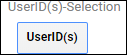
USER ID(S)
The training points can be filtered into the model results by selecting the initials of who digitized the points. This functionality also allows for choosing an individual’s training points by color. Once filtered, those points aren’t included into the model. As a result, this option is used to remove points that cannot be further adjusted outside the model envelope range (60%-110%).
Clicking the ‘UserID(s)’ button displays a list of users and colors for a state or ecoregion.

The default is ALL, meaning all points from all users, not particular user(s) or color(s), are used to run in the model. Either the ALL checkbox must be checked OR one or more users and colors can be selected.

Note that the user’s initials and colors can still be checked on and off if ‘ALL’ is selected. It will still use all colors and initial combinations unless ‘ALL’ is unchecked.

NOTE: When the UserID(s) button is used, the application must be restarted to use a different state or year.
3-Produce Results
In this section the model is run with the parameters from section one and two.

SAVE NAIP NATIVE SCALE
When the Save NAIP Native scale is checked, the NNS map and points will then populate in the tasks window after selecting ‘Run Model’. From there, they can run and be saved to permanent storage. The permanent storage location is projects/USFS/FHAAST/NAIP_DT/bioclimDB/ state / year

RUN MODEL
When the Run Model button is used, the model outputs are initiated and the BIOCLIM map(s) and points are added as layers for viewing on the map. The console window displays the envelope, overall accuracy and the kappa statistics for each color.
Select Run Model. Keep in mind that it’s necessary to view the model outputs on the map first before you save them. In the first model run, the ‘Save NAIP Native scale output’ checkbox should always remain unchecked.
Once ‘Run Model’ is clicked, the page will become unresponsive and appear frozen. After a while, a ‘Page Unresponsive’ prompt will appear. It’s best to select ‘Wait’ or leave the prompt on the screen until the page becomes responsive again. This process is interacting with GEE servers and requires a couple of minutes.

When the page becomes responsive again, the confirmation box seen below will display centered on the top of the map. The model run time is deceiving because at this point it’s still waiting to finish computing in the console window. Go ahead and press ‘Close’ and open the console window on the top right bar.

In the ‘Console’ window, it will display the model parameters set earlier. This includes the selected UserID(s), Total Point Size, NAIP Native Scale, Model Envelopes, Overall Accuracy, and Kappa Statistics. Scroll down below the sampleRegions line to view the model statistics.
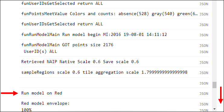
The accuracy and kappa statistics take a while to successfully compute. The spinning cog next to the ComputedObject line in the console will disappear once the statistics are complete, and will generate the ENV, Accuracy, and Kappa data. The overall accuracy reflects how precise the outputs are modeled. This range goes from zero to one and .50 would entail that the accuracy is a coin toss for modeling within the desired color space.

The finished computed layers will allow for the user to display them on the map from the ‘Layers’ dropdown window. Keep in mind, that the selected scale won’t draw on the map unless the viewed map scale is zoomed to 500 meters or less.


3.1-NOTES BEFORE RUNNING
The next steps are outside the GUI and are a bit awkward. The Forest Service has asked GEE for a function to replace these steps. Meanwhile the steps are the following:
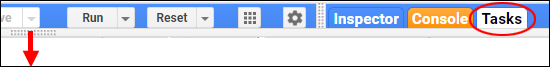
Click show code or drag the bar above the map to reveal the ‘Tasks’ tab at the top right.
Click ‘Run’ box to the right of the saved file.

Click ‘Run’ button on the displayed panel.

Running a task can require a lot of time to complete-from seconds to hours to days. Naip native scale will take longer amounts of time to finish running due to being a finer resolution, as opposed to running a coarser scale task (>nns), which will be a smaller file size and can finish quicker. Naip native scale will always be desired for exporting, whereas courser scales can be developed from the nns scale in a separate application known as the npiRescaler. While running, a spinning cog icon will rotate to the right of the export file name followed by the amount of time the task has been running.

The export file name will be highlighted in blue when the task is finished. It is safe to exit the application while the task is running.

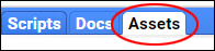
Once the task is complete, the file will be shown in the ‘Assets’ tab. Please note that it’s best to limit the number of tasks that are running at the same time. Multiple tasks prolong completion time.

4-Model Outputs
As many as three output maps are produced by this application. These are:
Native NAIP Scale Image
Selected Scale Image
Points
All maps are output in geographic WGS 84, EPSG 4326 rather than a projection so that mapping software can more quickly reproject on the fly to the desired output projection.
All displays have non-treed areas masked out from a 30-meter treed/non-treed map. The permanent storage maps do not have areas masked in the eventuality that higher quality non-treed maps might one day be produced.
The images are in five bands that coincide with the NPD application input training points. The points and the NAIP imagery are used as model input to produce the following output imagery in five bands:
| BAND | DESCRIPTION |
|---|---|
| Red | Red crowns on (typically) dying tree |
| Green | Green crowns on healthy tree |
| Gray | Gray crowns on (typically) dead tree |
| Absence | Gray to red rock, soils, or non-tree pixels |
| Shadow | Dark object or pixel that would normally have color, such as an area shaded by tree crown |
4.1-NATIVE NAIP SCALE IMAGE
A NNS image with cell values of presence(one) or absences(zero) cells for each of the five bands. The NNS is 0.6 or 1 meter and greater than one meter for years prior to 2014.
The image includes the computed envelope, accuracy and kappa statistics for each color.
4.2-SELECTED SCALE IMAGE
The selected scale image has cell values of zero to one hundred for each of the five bands. The value is the percentage of the cell that has the particular color. Scales of three or greater average the NNS cells to produce the percentage value in the reduced resolution image. The bands are displayed as a range of light (1%) to dark (100%) of a color on the map.
A green index layer is computed on the fly from the red, green and gray bands and provides a concise representation average for Tree Crown Health. The green index layer is derived by taking the mean value of total outputted pixel and calculated based on green minus red and gray outputs. This will only compute with a coarser scale that’s greater than Native naip scale. That’s primarily because it will average multiple outputs through a neighboring grid. An example here would be that a 30-meter scale is comprised by a 30 x 30 grid, and the average can then be classified within a range of 0 – 100. A percent threshold can then be color ramped and classified based on the percent of damage within that 30 x 30 Native naip grid.
The image includes the computed envelope, accuracy and kappa statistics for each color. This can be viewed by selecting the image asset file and opening its properties.
The properties of a saved asset file can be viewed reached by beginning to select the asset tab in GEE.
Following the Asset tab, scroll through the asset directory and select the USFS agency folder repository.
4.3-POINTS
The points have the following attributes that are captured in the NPD application: Note: A coarser sampleregion scale is set to the NNS for a state. This change will shift the training point within the NNS pixel and can make it off-centered. If sampleregion scale is set to greater than one, it will shift the training points drastically outside its original pixel.
| ATTRIBUTE | DESCRIPTION |
|---|---|
| ID | Sequential identifier for deleting |
| StatePostal | State postal code |
| EcoRegion | ID of selected eco region |
| UserID | User identifier |
| NaipYear | NAIP year |
| DateStartRange | Earliest date of imagery the user selected |
| DateEndRange | Last date of imagery the user selected |
| DateStartPixel | Earliest day on the selected pixel |
| DateEndPixel | Last day on the selected pixel |
| Color | Selected color either red, green, gray, absence, shadow |
The following additional attribute fields from the model are added to each point. Longitude and latitude coordinates are added as fields for ease of ingesting as a Comma Separated Value (CSV) file. The fields that are added are the following:
| ATTRIBUTE | DESCRIPTION |
|---|---|
| longitude | Longitude coordinate |
| latitude | Latitude coordinate |
| cv | Coefficient of variation in the NAIP Red, Green and Blue bands |
| mean | Mean of NAIP RGB bands |
| ndgb | Normalized difference in NAIP G and B bands |
| ndnb | Normalized difference in NAIP Near Infrared (N) and B bands |
| ndng | Normalized difference in NAIP N and G bands |
| ndrb | Normalized difference in NAIP R and B bands |
| ndrg | Normalized difference in NAIP R and G bands |
| ndvi | Normalized difference vegetation index |
| random | The random number assigned to each point during model development |
FAQ's
When a different state is selected that has the same most recent year a negative sign is placed on the choice so that the on-change event can fire and update the colors and user IDs. This possibly occurs when selecting a different state with the same most recent year in the same NPI session.
Zoom into the display. The one-meter BIOCLIM displays slowly but without errors. Zoom in extremely tight to display the selected meter size BIOCLIM to avoid errors such as:
It takes more memory to view outputs at a larger scale

A big state with a lot of points might cause this. Leave the panel alone or select wait to continue processing. Selecting Exit page will dismiss the application.

Use multiple browser tabs to see different states, years, colors or users.
This indicates that there are no pixel values being shown. It may resolve itself by changing the zoom level.
The npiRescaler application resamples Naip Native scale resolution and saves the reduced resolution image as an asset.